Spatio-temporal trend analysis of temperature using Python

Tutors: Alexander Kmoch1, Holger Virro1, and Evelyn Uuemaa1

1Landscape Geoinformatics Lab, Chair of Geoinformatics, Department of Geography, University of Tartu

Introduction

Under the climate change threat, we need to quantify the spatio-temporal trend of temperature and rainfall patterns to understand and evaluate the potential impacts of climate change on ecosystem services, energy fluxes and biogeochemical processes. There are wide range of global or regional scale climate data freely available in a gridded format that can be used for spatio-temporal analysis. These data can be derived directly from satellite remote sensing data or based on reanalysis of weather station time series data. Additionally, some gridded data are also developed by combining time series data from weather stations with remote sensing data.

Aim of the workshop

The goal of this session is to teach the participants how to handle NetCDF datasets, apply the Mann-Kendall (MK) test and calculate Sen’s slope (SS) values on a gridded climate dataset (please, check additional info below).

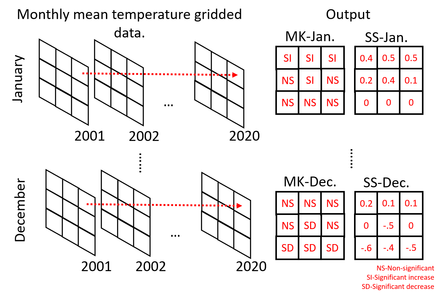
We will use the gridded daily mean temperature product from European Climate Assessment and Dataset (E-OBS version v23.1e) (Cornes et al., 2018). E-OBS is developed by interpolating climate data from weather stations provided by the national meteorological agencies of the European countries. The product is available at a grid resolution of 0.1° or 0.25° and covers the period since 1950 to present. For the workshop, we will use the 0.1° resolution dataset (which represents a resolution of about 11 km at the equator) from January 2001 until December 2020 already aggregated into monthly mean temperature (°C). The figure below illustrates how we will calculate MK and SS at pixel scale on monthly basis.

Mann-Kendall test for trend analysis

Different methodologies have combined spatial data sets and nonparametric statistical methods, such as the Mann-Kendall (MK) (Mann, 1945; Kendall, 1957) test, to infer about the temporal trends of climatic variables time series (Atta-ur-Rahman and Dawood, 2017; Jaagus et al., 2017; Silva Junior et al., 2018). As MK is a nonparametric test, it does not require normal distribution of the data, but it does assume no autocorrelation in the time series.

The MK test has as null hypothesis that the time series has no trend, and the alternative hypothesis is that it does have a trend (upward or downward). The test first calculates the differences between all pairs of earlier and later data points in the time series. After that, it calculates the variance of these differences, which is posteriorly used to calculate the Z test value. Finally, the statistical significance of the trend is quantified by calculating the probability associated with the normalized Z test. If $Z>0$, it indicates an increasing trend and if $Z<0$ it indicates a decreasing trend. Usually, the trends are defined as significant using 95% confidence level.

In addition to the trend calculation, it is also possible to quantify the magnitude of the trends. The magnitudes can be estimated by using the nonparametric Sen statistic, more specifically, the Theil–Sen estimator (Sen Pranab Kumar, 1968), which is given by the median of the slopes of each pair of points. To calculate the Sen’s slope, the times series data is ordered accordingly to the time (as function of time) and a confidence interval is provided for each slope value (same as in the MK test).

NetCDF files

NetCDF is a file format that allows the storage of multidimensional data into a single file archive and has been widely used. Check more info about NetCDF and Python by following this YouTube tutorial produced by Copernicus Marine Service.

Reading the NetCDF file with Xarray

We will start by importing all Python libraries used in this workshop. Data loading will be handled by Intake. For data processing and wrangling we are going to use the Xarray, Pandas and NumPy libraries. Matplotlib will be used for plotting purposes. Trend analysis will be carried out using the pyMannKendall library.

# Import libraries

# Data loading
import intake
import intake_xarray # Xarray wrapper for Intake
import h5netcdf # for NetCDF reading

# Processing
import xarray as xr
import pandas as pd
import numpy as np
import rioxarray # for CRS management in Xarray

# Trend analysis
import pymannkendall as mk

# Plotting
import matplotlib
import matplotlib.pyplot as plt
import matplotlib.colors as mcolors
import collections
import matplotlib.patches as mpatches
import calendar

Our prepared (smaller) NetCDF data files are located in the online workshop GitHub repository and the file’s metadata is given in another online metadata file, workshop_catalog.yaml, also located in the workshop’s GitHub repository.

print('https://raw.githubusercontent.com/LandscapeGeoinformatics/biogeomon_2022_pangeo/main/resources/workshop_catalog.yaml')

https://raw.githubusercontent.com/LandscapeGeoinformatics/biogeomon_2022_pangeo/main/resources/workshop_catalog.yaml

Let us open the catalog file and list its content. We will use the Intake library for loading the data. It allows for convenient data import from external locations.

# Open catalog file
cat = intake.open_catalog('https://raw.githubusercontent.com/LandscapeGeoinformatics/biogeomon_2022_pangeo/main/resources/workshop_catalog.yaml')
list(cat)

['monthly_precip_baltics', 'monthly_temp_baltics']

We are going to use only the temperature file named monthly_temp_baltics.nc in this workshop. First, let us see the metadata of this NetCDF.

# Read metadata
temp_data = cat.monthly_temp_baltics
temp_data

monthly_temp_baltics:
  args:
    urlpath: https://github.com/LandscapeGeoinformatics/biogeomon_2022_pangeo/raw/main/resources/monthly_temp_baltics.nc
  description: Monthly temperature data for the Baltics
  driver: intake_xarray.netcdf.NetCDFSource
  metadata:
    catalog_dir: https://raw.githubusercontent.com/LandscapeGeoinformatics/biogeomon_2022_pangeo/main/resources

The metadata includes the parameters * urlpath showing the location of the NetCDF * the description of the data * driver to be used when importing the data * catalog_dir showing the catalog file location

Now we can read the NetCDF with monthly temperature data for the Baltic states in the period 2001–2020. We are going to read the data as an Xarray dataset. The Xarray library allows for convenient manipulation of multidimensional arrays and interaction with the two main data objects—DataArray and Dataset—borrows elements from the Rasterio, Pandas and NumPy Python libraries.

Xarray is a part of the Pangeo big data geoscience environment and is particularly useful for working with large datasets. As our dataset is not quite that big, we will only use some of the main Xarray functionalities for our analysis.

As the driver used for reading the file is already specified in the catalog, we can simply use read to import the temperature data.

# Import temperature data as an Xarray dataset
temp_ds = temp_data.read()
temp_ds

<xarray.Dataset>
Dimensions:      (latitude: 57, longitude: 72, ym: 240)
Coordinates:
  * latitude     (latitude) float64 53.95 54.05 54.15 ... 59.35 59.45 59.55
  * longitude    (longitude) float64 21.05 21.15 21.25 ... 27.95 28.05 28.15
  * ym           (ym) object '2001-01' '2001-02' ... '2020-11' '2020-12'
    spatial_ref  int32 0
Data variables:
    temp_mean    (latitude, longitude, ym) float32 nan nan nan ... nan nan nan
Attributes:
    grid_mapping:  spatial_ref

xarray.Dataset

• Dimensions:
  • latitude: 57
  • longitude: 72
  • ym: 240
• Coordinates: (4)
  • latitude
    (latitude)
    float64
    53.95 54.05 54.15 ... 59.45 59.55

    array([53.949861, 54.049861, 54.149861, 54.249861, 54.349861, 54.449861,
           54.549861, 54.649861, 54.749861, 54.849861, 54.949861, 55.049861,
           55.149861, 55.249861, 55.349861, 55.449861, 55.549861, 55.649861,
           55.749861, 55.849861, 55.949861, 56.049861, 56.149861, 56.249861,
           56.349861, 56.449861, 56.549861, 56.649861, 56.749861, 56.849861,
           56.949861, 57.049861, 57.149861, 57.249861, 57.349861, 57.449861,
           57.549861, 57.649861, 57.749861, 57.849861, 57.949861, 58.049861,
           58.149861, 58.249861, 58.349861, 58.449861, 58.549861, 58.649861,
           58.749861, 58.849861, 58.949861, 59.049861, 59.149861, 59.249861,
           59.349861, 59.449861, 59.549861])

  • longitude
    (longitude)
    float64
    21.05 21.15 21.25 ... 28.05 28.15

    array([21.04986, 21.14986, 21.24986, 21.34986, 21.44986, 21.54986, 21.64986,
           21.74986, 21.84986, 21.94986, 22.04986, 22.14986, 22.24986, 22.34986,
           22.44986, 22.54986, 22.64986, 22.74986, 22.84986, 22.94986, 23.04986,
           23.14986, 23.24986, 23.34986, 23.44986, 23.54986, 23.64986, 23.74986,
           23.84986, 23.94986, 24.04986, 24.14986, 24.24986, 24.34986, 24.44986,
           24.54986, 24.64986, 24.74986, 24.84986, 24.94986, 25.04986, 25.14986,
           25.24986, 25.34986, 25.44986, 25.54986, 25.64986, 25.74986, 25.84986,
           25.94986, 26.04986, 26.14986, 26.24986, 26.34986, 26.44986, 26.54986,
           26.64986, 26.74986, 26.84986, 26.94986, 27.04986, 27.14986, 27.24986,
           27.34986, 27.44986, 27.54986, 27.64986, 27.74986, 27.84986, 27.94986,
           28.04986, 28.14986])

  • ym
    (ym)
    object
    '2001-01' '2001-02' ... '2020-12'

    array(['2001-01', '2001-02', '2001-03', ..., '2020-10', '2020-11', '2020-12'],
          dtype=object)

  • spatial_ref
    ()
    int32
    0

    crs_wkt :

    GEOGCS["WGS 84",DATUM["WGS_1984",SPHEROID["WGS 84",6378137,298.257223563,AUTHORITY["EPSG","7030"]],AUTHORITY["EPSG","6326"]],PRIMEM["Greenwich",0,AUTHORITY["EPSG","8901"]],UNIT["degree",0.0174532925199433,AUTHORITY["EPSG","9122"]],AXIS["Latitude",NORTH],AXIS["Longitude",EAST],AUTHORITY["EPSG","4326"]]

    semi_major_axis :

    6378137.0

    semi_minor_axis :

    6356752.314245179

    inverse_flattening :

    298.257223563

    reference_ellipsoid_name :

    WGS 84

    longitude_of_prime_meridian :

    0.0

    prime_meridian_name :

    Greenwich

    geographic_crs_name :

    WGS 84

    grid_mapping_name :

    latitude_longitude

    spatial_ref :

    GEOGCS["WGS 84",DATUM["WGS_1984",SPHEROID["WGS 84",6378137,298.257223563,AUTHORITY["EPSG","7030"]],AUTHORITY["EPSG","6326"]],PRIMEM["Greenwich",0,AUTHORITY["EPSG","8901"]],UNIT["degree",0.0174532925199433,AUTHORITY["EPSG","9122"]],AXIS["Latitude",NORTH],AXIS["Longitude",EAST],AUTHORITY["EPSG","4326"]]

    array(0)

• Data variables: (1)
  • temp_mean
    (latitude, longitude, ym)
    float32
    nan nan nan nan ... nan nan nan nan

    grid_mapping :

    spatial_ref

    array([[[        nan,         nan,         nan, ...,         nan,
                     nan,         nan],
            [        nan,         nan,         nan, ...,         nan,
                     nan,         nan],
            [        nan,         nan,         nan, ...,         nan,
                     nan,         nan],
            ...,
            [        nan,         nan,         nan, ...,         nan,
                     nan,         nan],
            [        nan,         nan,         nan, ...,         nan,
                     nan,         nan],
            [        nan,         nan,         nan, ...,         nan,
                     nan,         nan]],
    
           [[        nan,         nan,         nan, ...,         nan,
                     nan,         nan],
            [        nan,         nan,         nan, ...,         nan,
                     nan,         nan],
            [        nan,         nan,         nan, ...,         nan,
                     nan,         nan],
    ...
            [        nan,         nan,         nan, ...,         nan,
                     nan,         nan],
            [-1.7364515 , -6.0203576 , -3.3258066 , ...,  8.616452  ,
              3.806333  , -0.85096776],
            [        nan,         nan,         nan, ...,         nan,
                     nan,         nan]],
    
           [[        nan,         nan,         nan, ...,         nan,
                     nan,         nan],
            [        nan,         nan,         nan, ...,         nan,
                     nan,         nan],
            [        nan,         nan,         nan, ...,         nan,
                     nan,         nan],
            ...,
            [        nan,         nan,         nan, ...,         nan,
                     nan,         nan],
            [        nan,         nan,         nan, ...,         nan,
                     nan,         nan],
            [        nan,         nan,         nan, ...,         nan,
                     nan,         nan]]], dtype=float32)

• Attributes: (1)

  grid_mapping :

  spatial_ref

Our dataset has three dimensions, each of which has their own set of coordinates. The spatial dimension is made up of 57 latitude and 72 longitude coordinates, meaning that there are a total of $57\times 72=4104$ unique locations with temperature information in the grid. Third dimension ym is an array of all 240 year–month pairs (e.g. 2001-01) covering the 20 year study period.

The fourth coordinate spatial_ref is not a separate dimension, but an indicator that a coordinate reference system (CRS) has been assigned to the data. The grid_mapping attribute of this fourth coordinate holds information about the CRS of the dataset. If we display the attrs property then we can see that the CRS in this case is WGS84.

# Display CRS information
display(temp_ds['spatial_ref'].attrs)

{'crs_wkt': 'GEOGCS["WGS 84",DATUM["WGS_1984",SPHEROID["WGS 84",6378137,298.257223563,AUTHORITY["EPSG","7030"]],AUTHORITY["EPSG","6326"]],PRIMEM["Greenwich",0,AUTHORITY["EPSG","8901"]],UNIT["degree",0.0174532925199433,AUTHORITY["EPSG","9122"]],AXIS["Latitude",NORTH],AXIS["Longitude",EAST],AUTHORITY["EPSG","4326"]]',
 'semi_major_axis': 6378137.0,
 'semi_minor_axis': 6356752.314245179,
 'inverse_flattening': 298.257223563,
 'reference_ellipsoid_name': 'WGS 84',
 'longitude_of_prime_meridian': 0.0,
 'prime_meridian_name': 'Greenwich',
 'geographic_crs_name': 'WGS 84',
 'grid_mapping_name': 'latitude_longitude',
 'spatial_ref': 'GEOGCS["WGS 84",DATUM["WGS_1984",SPHEROID["WGS 84",6378137,298.257223563,AUTHORITY["EPSG","7030"]],AUTHORITY["EPSG","6326"]],PRIMEM["Greenwich",0,AUTHORITY["EPSG","8901"]],UNIT["degree",0.0174532925199433,AUTHORITY["EPSG","9122"]],AXIS["Latitude",NORTH],AXIS["Longitude",EAST],AUTHORITY["EPSG","4326"]]'}

Data variable temp_mean contains the monthly temperature amounts of the Baltics in the period 2001–2020. Since each unique location has a time series length of 240 months, the variable contains a total of $57\times 72\times 240=984960$ values.

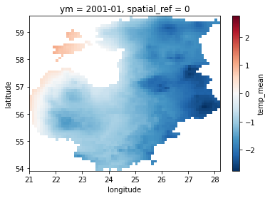
For a quick visualization of our data, let us plot the temperature amount for January 2001. We can use the sel function and specify the specific month by using the corresponding coordinate ym. We also need to include the data variable temp_mean to our plotting call.

# Select a specific month
temp_ds.sel(ym='2001-01')

<xarray.Dataset>
Dimensions:      (latitude: 57, longitude: 72)
Coordinates:
  * latitude     (latitude) float64 53.95 54.05 54.15 ... 59.35 59.45 59.55
  * longitude    (longitude) float64 21.05 21.15 21.25 ... 27.95 28.05 28.15
    ym           <U7 '2001-01'
    spatial_ref  int32 0
Data variables:
    temp_mean    (latitude, longitude) float32 nan nan nan nan ... nan nan nan
Attributes:
    grid_mapping:  spatial_ref

xarray.Dataset

• Dimensions:
  • latitude: 57
  • longitude: 72
• Coordinates: (4)
  • latitude
    (latitude)
    float64
    53.95 54.05 54.15 ... 59.45 59.55

    array([53.949861, 54.049861, 54.149861, 54.249861, 54.349861, 54.449861,
           54.549861, 54.649861, 54.749861, 54.849861, 54.949861, 55.049861,
           55.149861, 55.249861, 55.349861, 55.449861, 55.549861, 55.649861,
           55.749861, 55.849861, 55.949861, 56.049861, 56.149861, 56.249861,
           56.349861, 56.449861, 56.549861, 56.649861, 56.749861, 56.849861,
           56.949861, 57.049861, 57.149861, 57.249861, 57.349861, 57.449861,
           57.549861, 57.649861, 57.749861, 57.849861, 57.949861, 58.049861,
           58.149861, 58.249861, 58.349861, 58.449861, 58.549861, 58.649861,
           58.749861, 58.849861, 58.949861, 59.049861, 59.149861, 59.249861,
           59.349861, 59.449861, 59.549861])

  • longitude
    (longitude)
    float64
    21.05 21.15 21.25 ... 28.05 28.15

    array([21.04986, 21.14986, 21.24986, 21.34986, 21.44986, 21.54986, 21.64986,
           21.74986, 21.84986, 21.94986, 22.04986, 22.14986, 22.24986, 22.34986,
           22.44986, 22.54986, 22.64986, 22.74986, 22.84986, 22.94986, 23.04986,
           23.14986, 23.24986, 23.34986, 23.44986, 23.54986, 23.64986, 23.74986,
           23.84986, 23.94986, 24.04986, 24.14986, 24.24986, 24.34986, 24.44986,
           24.54986, 24.64986, 24.74986, 24.84986, 24.94986, 25.04986, 25.14986,
           25.24986, 25.34986, 25.44986, 25.54986, 25.64986, 25.74986, 25.84986,
           25.94986, 26.04986, 26.14986, 26.24986, 26.34986, 26.44986, 26.54986,
           26.64986, 26.74986, 26.84986, 26.94986, 27.04986, 27.14986, 27.24986,
           27.34986, 27.44986, 27.54986, 27.64986, 27.74986, 27.84986, 27.94986,
           28.04986, 28.14986])

  • ym
    ()
    <U7
    '2001-01'

    array('2001-01', dtype='<U7')

  • spatial_ref
    ()
    int32
    0

    crs_wkt :

    GEOGCS["WGS 84",DATUM["WGS_1984",SPHEROID["WGS 84",6378137,298.257223563,AUTHORITY["EPSG","7030"]],AUTHORITY["EPSG","6326"]],PRIMEM["Greenwich",0,AUTHORITY["EPSG","8901"]],UNIT["degree",0.0174532925199433,AUTHORITY["EPSG","9122"]],AXIS["Latitude",NORTH],AXIS["Longitude",EAST],AUTHORITY["EPSG","4326"]]

    semi_major_axis :

    6378137.0

    semi_minor_axis :

    6356752.314245179

    inverse_flattening :

    298.257223563

    reference_ellipsoid_name :

    WGS 84

    longitude_of_prime_meridian :

    0.0

    prime_meridian_name :

    Greenwich

    geographic_crs_name :

    WGS 84

    grid_mapping_name :

    latitude_longitude

    spatial_ref :

    GEOGCS["WGS 84",DATUM["WGS_1984",SPHEROID["WGS 84",6378137,298.257223563,AUTHORITY["EPSG","7030"]],AUTHORITY["EPSG","6326"]],PRIMEM["Greenwich",0,AUTHORITY["EPSG","8901"]],UNIT["degree",0.0174532925199433,AUTHORITY["EPSG","9122"]],AXIS["Latitude",NORTH],AXIS["Longitude",EAST],AUTHORITY["EPSG","4326"]]

    array(0)

• Data variables: (1)
  • temp_mean
    (latitude, longitude)
    float32
    nan nan nan nan ... nan nan nan nan

    grid_mapping :

    spatial_ref

    array([[       nan,        nan,        nan, ...,        nan,        nan,
                   nan],
           [       nan,        nan,        nan, ...,        nan,        nan,
                   nan],
           [       nan,        nan,        nan, ...,        nan,        nan,
                   nan],
           ...,
           [       nan,        nan,        nan, ..., -1.7796775, -1.7503226,
            -1.7583872],
           [       nan,        nan,        nan, ...,        nan, -1.7364515,
                   nan],
           [       nan,        nan,        nan, ...,        nan,        nan,
                   nan]], dtype=float32)

• Attributes: (1)

  grid_mapping :

  spatial_ref

# Select and plot a specific month
temp_ds.sel(ym='2001-01')['temp_mean'].plot()

<matplotlib.collections.QuadMesh at 0x19f3be9ce80>

Getting data ready for trend analysis

Now that we have familiarized ourselves with the dataset, let us prepare it for trend analysis.

This preprocessing phase will consist of * Converting the Xarray Dataset into a Pandas DataFrame * Grouping the data by location (grid cell) and month * Extracting the grouped temperature values as a NumPy array

We will start by converting the dataset into a Pandas DataFrame using the corresponding function to_dataframe. Using reset_index will flatten the DataFrame, so that we have a separate row for each of our 984960 monthly temperature records.

# Convert the xarray to Pandas DF
temp_df = temp_ds.to_dataframe().reset_index() # flatten
display(temp_df)

	latitude	longitude	ym	temp_mean	spatial_ref
0	53.949861	21.04986	2001-01	NaN	0
1	53.949861	21.04986	2001-02	NaN	0
2	53.949861	21.04986	2001-03	NaN	0
3	53.949861	21.04986	2001-04	NaN	0
4	53.949861	21.04986	2001-05	NaN	0
...	...	...	...	...	...
984955	59.549861	28.14986	2020-08	NaN	0
984956	59.549861	28.14986	2020-09	NaN	0
984957	59.549861	28.14986	2020-10	NaN	0
984958	59.549861	28.14986	2020-11	NaN	0
984959	59.549861	28.14986	2020-12	NaN	0

984960 rows × 5 columns

The input data includes a large number of missing values, indicated by NaN in the temp_mean column. These are grid cells located outside the study area (i.e. the Baltic Sea, neighboring countries).

We should remove them with dropna before moving on.

# Drop rows with missing temperature values
temp_df = temp_df.dropna().reset_index()
temp_df

	index	latitude	longitude	ym	temp_mean	spatial_ref
0	6000	53.949861	23.54986	2001-01	-1.155484	0
1	6001	53.949861	23.54986	2001-02	-2.777500	0
2	6002	53.949861	23.54986	2001-03	0.088065	0
3	6003	53.949861	23.54986	2001-04	8.223666	0
4	6004	53.949861	23.54986	2001-05	13.019676	0
...	...	...	...	...	...	...
611275	980635	59.549861	26.34986	2020-08	16.812258	0
611276	980636	59.549861	26.34986	2020-09	13.711668	0
611277	980637	59.549861	26.34986	2020-10	9.299999	0
611278	980638	59.549861	26.34986	2020-11	5.165666	0
611279	980639	59.549861	26.34986	2020-12	0.163548	0

611280 rows × 6 columns

Let us also split the ym column into separate year and month columns for more convenient grouping later on. We can use the function split for that and specify the delimiter in the original column.

# Extract year and month from the observation date as new columns
temp_df[['year', 'month']] = temp_df['ym'].str.split('-', expand=True) # expand=True tells Pandas that there are two output columns
temp_df['year'] = temp_df['year'].astype(int) # astype(int) will convert string column into integer
temp_df['month'] = temp_df['month'].astype(int)
display(temp_df)

	index	latitude	longitude	ym	temp_mean	spatial_ref	year	month
0	6000	53.949861	23.54986	2001-01	-1.155484	0	2001	1
1	6001	53.949861	23.54986	2001-02	-2.777500	0	2001	2
2	6002	53.949861	23.54986	2001-03	0.088065	0	2001	3
3	6003	53.949861	23.54986	2001-04	8.223666	0	2001	4
4	6004	53.949861	23.54986	2001-05	13.019676	0	2001	5
...	...	...	...	...	...	...	...	...
611275	980635	59.549861	26.34986	2020-08	16.812258	0	2020	8
611276	980636	59.549861	26.34986	2020-09	13.711668	0	2020	9
611277	980637	59.549861	26.34986	2020-10	9.299999	0	2020	10
611278	980638	59.549861	26.34986	2020-11	5.165666	0	2020	11
611279	980639	59.549861	26.34986	2020-12	0.163548	0	2020	12

611280 rows × 8 columns

In order to make sure that the monthly temperature values end up in the correct order during grouping we should sort the DataFrame by year and month. This can be done using the sort_values function.

# Sort the DataFrame by year and month in ascending order
temp_df.sort_values(['year', 'month'], ascending=[True, True], inplace=True) # inplace=True tells Pandas to modify the existing object

Now we can aggregate the DataFrame by location and month. We will use groupby to determine the columns used for grouping and assign temp_mean as the target column.

Pandas function apply can be used for applying different functions rowwise in a DataFrame. In this case, we use parameter np.array to tell apply to collect the grouped temperature values into a NumPy array for each row.

# Group locations by month and collect observation values to NumPy array
temp_group_df = temp_df\
    .groupby(['latitude', 'longitude', 'month'])['temp_mean']\
    .apply(np.array)\
    .reset_index() # flatten the DataFrame
display(temp_group_df)

	latitude	longitude	month	temp_mean
0	53.949861	23.54986	1	[-1.155484, -1.569032, -5.0525813, -6.9348392,...
1	53.949861	23.54986	2	[-2.7775, 2.2021434, -6.039285, -1.8844824, -5...
2	53.949861	23.54986	3	[0.08806454, 3.3738706, 0.8622579, 1.8580645, ...
3	53.949861	23.54986	4	[8.223666, 8.266, 5.5366664, 7.551, 7.8069997,...
4	53.949861	23.54986	5	[13.019676, 15.822902, 14.108708, 10.822258, 1...
...	...	...	...	...
30559	59.549861	26.34986	8	[15.805161, 18.406773, 16.10516, 17.048388, 16...
30560	59.549861	26.34986	9	[12.335667, 11.58, 11.987667, 12.545667, 13.21...
30561	59.549861	26.34986	10	[8.4554825, 1.8396775, 4.703548, 6.5590324, 7....
30562	59.549861	26.34986	11	[0.766, -1.2219999, 2.9746668, 0.9679999, 3.94...
30563	59.549861	26.34986	12	[-6.6154838, -7.694516, 0.27806458, 0.46129018...

30564 rows × 4 columns

Let us check the cell content in the array column for the first row. It contains 20 years worth of monthly temperature mean values for January at 53.9499 latitude and 23.5499 longitude.

We can use iloc to select a DataFrame row by index.

# Display first row
display(temp_group_df.iloc[0])

# Display cell content in the grouped column
display(temp_group_df.iloc[0]['temp_mean'])

latitude                                             53.949861
longitude                                             23.54986
month                                                        1
temp_mean    [-1.155484, -1.569032, -5.0525813, -6.9348392,...
Name: 0, dtype: object

array([ -1.155484  ,  -1.569032  ,  -5.0525813 ,  -6.9348392 ,
        -0.04483882,  -7.9774194 ,   1.5177417 ,  -0.8593547 ,
        -3.7196774 , -10.487097  ,  -2.7848382 ,  -3.04      ,
        -5.996774  ,  -5.3016133 ,  -0.33290324,  -5.7196774 ,
        -4.384839  ,  -1.638387  ,  -4.256451  ,   2.0070968 ],
      dtype=float32)

Trend analysis using the Mann-Kendall (MK) test

Now we have the temperature arrays in a column and can move on with the trend analysis. We are going to use the pyMannKendall library for that.

Although there are 13 different versions of the MK test available in pyMannKendall, the original_test will suffice for now.

The test will return a tuple containing the named parameters * trend: tells the trend (increasing, decreasing or no trend) * h: True (if trend is present) or False (if the trend is absence) * p: p-value of the significance test * z: normalized test statistics * Tau: Kendall Tau * s: Mann-Kendal’s score * var_s: Variance S * slope: Theil-Sen estimator/slope * intercept: intercept of Kendall-Theil Robust Line

# Check the ouput of the MK test function
array = temp_group_df.iloc[0]['temp_mean']
result = mk.original_test(array, alpha=0.05)
display(result)

Mann_Kendall_Test(trend='no trend', h=False, p=0.9741177473553713, z=0.03244428422615251, Tau=0.010526315789473684, s=2.0, var_s=950.0, slope=0.03997344138858082, intercept=-3.759586398254384)

We will loop over the arrays in the temp_mean column, applying the MK test each time using apply. Confidence level—0.05 in our case—can be assigned with parameter alpha.

This can take some time as we need to repeat the process as many times as there are rows, i.e. 30564 iterations in total.

%%time
# Apply MK test rowwise and collect result into new column
temp_group_df['result'] = temp_group_df['temp_mean'].apply(lambda x: mk.original_test(x, alpha=0.05))
display(temp_group_df)

	latitude	longitude	month	temp_mean	result
0	53.949861	23.54986	1	[-1.155484, -1.569032, -5.0525813, -6.9348392,...	(no trend, False, 0.9741177473553713, 0.032444...
1	53.949861	23.54986	2	[-2.7775, 2.2021434, -6.039285, -1.8844824, -5...	(no trend, False, 0.2299690777236405, 1.200438...
2	53.949861	23.54986	3	[0.08806454, 3.3738706, 0.8622579, 1.8580645, ...	(no trend, False, 0.2299690777236405, 1.200438...
3	53.949861	23.54986	4	[8.223666, 8.266, 5.5366664, 7.551, 7.8069997,...	(no trend, False, 0.7702877264736667, 0.291998...
4	53.949861	23.54986	5	[13.019676, 15.822902, 14.108708, 10.822258, 1...	(no trend, False, 0.9741177473553713, 0.032444...
...	...	...	...	...	...
30559	59.549861	26.34986	8	[15.805161, 18.406773, 16.10516, 17.048388, 16...	(no trend, False, 0.721176307474874, 0.3568871...
30560	59.549861	26.34986	9	[12.335667, 11.58, 11.987667, 12.545667, 13.21...	(no trend, False, 0.07435290536856365, 1.78443...
30561	59.549861	26.34986	10	[8.4554825, 1.8396775, 4.703548, 6.5590324, 7....	(no trend, False, 0.5376032363488861, 0.616441...
30562	59.549861	26.34986	11	[0.766, -1.2219999, 2.9746668, 0.9679999, 3.94...	(no trend, False, 0.07435290536856365, 1.78443...
30563	59.549861	26.34986	12	[-6.6154838, -7.694516, 0.27806458, 0.46129018...	(no trend, False, 0.18344722817247305, 1.33021...

30564 rows × 5 columns

CPU times: total: 45.2 s
Wall time: 45.6 s

For our purposes, we will only extract parameters trend, p and slope, which have the indices 0, 2 and 7, respectively. We can use these indices to extract the parameters into separate columns from the MK test result column.

temp_group_df['trend'] = temp_group_df['result'].apply(lambda x: x[0])
temp_group_df['p'] = temp_group_df['result'].apply(lambda x: x[2])
temp_group_df['slope'] = temp_group_df['result'].apply(lambda x: x[7])
temp_group_df

	latitude	longitude	month	temp_mean	result	trend	p	slope
0	53.949861	23.54986	1	[-1.155484, -1.569032, -5.0525813, -6.9348392,...	(no trend, False, 0.9741177473553713, 0.032444...	no trend	0.974118	0.039973
1	53.949861	23.54986	2	[-2.7775, 2.2021434, -6.039285, -1.8844824, -5...	(no trend, False, 0.2299690777236405, 1.200438...	no trend	0.229969	0.251141
2	53.949861	23.54986	3	[0.08806454, 3.3738706, 0.8622579, 1.8580645, ...	(no trend, False, 0.2299690777236405, 1.200438...	no trend	0.229969	0.135081
3	53.949861	23.54986	4	[8.223666, 8.266, 5.5366664, 7.551, 7.8069997,...	(no trend, False, 0.7702877264736667, 0.291998...	no trend	0.770288	0.012048
4	53.949861	23.54986	5	[13.019676, 15.822902, 14.108708, 10.822258, 1...	(no trend, False, 0.9741177473553713, 0.032444...	no trend	0.974118	0.000922
...	...	...	...	...	...	...	...	...
30559	59.549861	26.34986	8	[15.805161, 18.406773, 16.10516, 17.048388, 16...	(no trend, False, 0.721176307474874, 0.3568871...	no trend	0.721176	0.018852
30560	59.549861	26.34986	9	[12.335667, 11.58, 11.987667, 12.545667, 13.21...	(no trend, False, 0.07435290536856365, 1.78443...	no trend	0.074353	0.066889
30561	59.549861	26.34986	10	[8.4554825, 1.8396775, 4.703548, 6.5590324, 7....	(no trend, False, 0.5376032363488861, 0.616441...	no trend	0.537603	0.042174
30562	59.549861	26.34986	11	[0.766, -1.2219999, 2.9746668, 0.9679999, 3.94...	(no trend, False, 0.07435290536856365, 1.78443...	no trend	0.074353	0.129285
30563	59.549861	26.34986	12	[-6.6154838, -7.694516, 0.27806458, 0.46129018...	(no trend, False, 0.18344722817247305, 1.33021...	no trend	0.183447	0.145511

30564 rows × 8 columns

We can use Pandas function value_counts to display how many grid cells ended up in each of the trend classes. We will do this for each month, so we are going to group temp_group_df again by month and loop through it.

# Loop through months and display significant trend count
for month, df in temp_group_df.groupby('month'):
    print('Siginificant trends in month number ' + str(month))
    display(df['trend'].value_counts())
    print('\n')

Siginificant trends in month number 1

no trend    2547
Name: trend, dtype: int64

Siginificant trends in month number 2

no trend    2547
Name: trend, dtype: int64

Siginificant trends in month number 3

no trend    2547
Name: trend, dtype: int64

Siginificant trends in month number 4

no trend      2536
increasing      11
Name: trend, dtype: int64

Siginificant trends in month number 5

no trend    2547
Name: trend, dtype: int64

Siginificant trends in month number 6

no trend      1531
increasing    1016
Name: trend, dtype: int64

Siginificant trends in month number 7

no trend      2436
decreasing     111
Name: trend, dtype: int64

Siginificant trends in month number 8

no trend    2547
Name: trend, dtype: int64

Siginificant trends in month number 9

no trend      1589
increasing     958
Name: trend, dtype: int64

Siginificant trends in month number 10

no trend      2469
increasing      78
Name: trend, dtype: int64

Siginificant trends in month number 11

increasing    2067
no trend       480
Name: trend, dtype: int64

Siginificant trends in month number 12

no trend      2543
increasing       4
Name: trend, dtype: int64

We can see that a large majority of locations did not show a significant trend during the study period as most cells indicated no trend.

Next we will convert the parameter trend into a new numeric column, which is required for plotting later on.

Let us first create a function that assigns a new numeric trend class based on p and slope. Negative significant trends will be indicated by -1, positive trends by 1 and 0 will be assigned to locations where no trend was detected.

# Function for numeric trend conversion
def numeric_trend(slope, p):
    if slope < 0 and p < 0.05:
        return -1
    elif slope > 0 and p < 0.05:
        return 1
    else:
        return 0

Now we can use apply and its lambda parameter to generate the numeric_trend column. The lambda parameter is useful for applying a function to each row.

In our case, we are taking the values of columns slope and p for each row as input parameters for our function numeric_trend, which we created in the last step. Parameter axis=1 will tell the function that we are iterating over rows rather than columns.

Some examples of lambda use can be found at https://pandas.pydata.org/docs/reference/api/pandas.DataFrame.apply.html.

# Create a numeric version of the trend column
temp_group_df['numeric_trend'] = temp_group_df.apply(lambda x: numeric_trend(x['slope'], x['p']), axis=1)
display(temp_group_df)

	latitude	longitude	month	temp_mean	result	trend	p	slope	numeric_trend
0	53.949861	23.54986	1	[-1.155484, -1.569032, -5.0525813, -6.9348392,...	(no trend, False, 0.9741177473553713, 0.032444...	no trend	0.974118	0.039973	0
1	53.949861	23.54986	2	[-2.7775, 2.2021434, -6.039285, -1.8844824, -5...	(no trend, False, 0.2299690777236405, 1.200438...	no trend	0.229969	0.251141	0
2	53.949861	23.54986	3	[0.08806454, 3.3738706, 0.8622579, 1.8580645, ...	(no trend, False, 0.2299690777236405, 1.200438...	no trend	0.229969	0.135081	0
3	53.949861	23.54986	4	[8.223666, 8.266, 5.5366664, 7.551, 7.8069997,...	(no trend, False, 0.7702877264736667, 0.291998...	no trend	0.770288	0.012048	0
4	53.949861	23.54986	5	[13.019676, 15.822902, 14.108708, 10.822258, 1...	(no trend, False, 0.9741177473553713, 0.032444...	no trend	0.974118	0.000922	0
...	...	...	...	...	...	...	...	...	...
30559	59.549861	26.34986	8	[15.805161, 18.406773, 16.10516, 17.048388, 16...	(no trend, False, 0.721176307474874, 0.3568871...	no trend	0.721176	0.018852	0
30560	59.549861	26.34986	9	[12.335667, 11.58, 11.987667, 12.545667, 13.21...	(no trend, False, 0.07435290536856365, 1.78443...	no trend	0.074353	0.066889	0
30561	59.549861	26.34986	10	[8.4554825, 1.8396775, 4.703548, 6.5590324, 7....	(no trend, False, 0.5376032363488861, 0.616441...	no trend	0.537603	0.042174	0
30562	59.549861	26.34986	11	[0.766, -1.2219999, 2.9746668, 0.9679999, 3.94...	(no trend, False, 0.07435290536856365, 1.78443...	no trend	0.074353	0.129285	0
30563	59.549861	26.34986	12	[-6.6154838, -7.694516, 0.27806458, 0.46129018...	(no trend, False, 0.18344722817247305, 1.33021...	no trend	0.183447	0.145511	0

30564 rows × 9 columns

Before plotting the trend results we need to convert our DataFrame back into an Xarray dataset. This can be done with to_xarray, but first we need to use set_index and assign an index to the DataFrame. The columns used for the index will end up as dimensions in the resulting Xarray dataset.

Let us also assign a CRS with write_crs from rioxarray, which is a supplementary Xarray library used for spatial operations.

# Convert the DataFrame back to xarray Dataset and assign CRS
temp_group_df.set_index(['latitude', 'longitude', 'month'], inplace=True)
temp_array = temp_group_df.to_xarray()
temp_array.rio.write_crs('epsg:4326', inplace=True)
display(temp_array)

<xarray.Dataset>
Dimensions:        (latitude: 57, longitude: 72, month: 12)
Coordinates:
  * latitude       (latitude) float64 53.95 54.05 54.15 ... 59.35 59.45 59.55
  * longitude      (longitude) float64 21.05 21.15 21.25 ... 27.95 28.05 28.15
  * month          (month) int64 1 2 3 4 5 6 7 8 9 10 11 12
    spatial_ref    int32 0
Data variables:
    temp_mean      (latitude, longitude, month) object nan nan nan ... nan nan
    result         (latitude, longitude, month) object nan nan nan ... nan nan
    trend          (latitude, longitude, month) object nan nan nan ... nan nan
    p              (latitude, longitude, month) float64 nan nan nan ... nan nan
    slope          (latitude, longitude, month) float64 nan nan nan ... nan nan
    numeric_trend  (latitude, longitude, month) float64 nan nan nan ... nan nan

xarray.Dataset

• Dimensions:
  • latitude: 57
  • longitude: 72
  • month: 12
• Coordinates: (4)
  • latitude
    (latitude)
    float64
    53.95 54.05 54.15 ... 59.45 59.55

    array([53.949861, 54.049861, 54.149861, 54.249861, 54.349861, 54.449861,
           54.549861, 54.649861, 54.749861, 54.849861, 54.949861, 55.049861,
           55.149861, 55.249861, 55.349861, 55.449861, 55.549861, 55.649861,
           55.749861, 55.849861, 55.949861, 56.049861, 56.149861, 56.249861,
           56.349861, 56.449861, 56.549861, 56.649861, 56.749861, 56.849861,
           56.949861, 57.049861, 57.149861, 57.249861, 57.349861, 57.449861,
           57.549861, 57.649861, 57.749861, 57.849861, 57.949861, 58.049861,
           58.149861, 58.249861, 58.349861, 58.449861, 58.549861, 58.649861,
           58.749861, 58.849861, 58.949861, 59.049861, 59.149861, 59.249861,
           59.349861, 59.449861, 59.549861])

  • longitude
    (longitude)
    float64
    21.05 21.15 21.25 ... 28.05 28.15

    array([21.04986, 21.14986, 21.24986, 21.34986, 21.44986, 21.54986, 21.64986,
           21.74986, 21.84986, 21.94986, 22.04986, 22.14986, 22.24986, 22.34986,
           22.44986, 22.54986, 22.64986, 22.74986, 22.84986, 22.94986, 23.04986,
           23.14986, 23.24986, 23.34986, 23.44986, 23.54986, 23.64986, 23.74986,
           23.84986, 23.94986, 24.04986, 24.14986, 24.24986, 24.34986, 24.44986,
           24.54986, 24.64986, 24.74986, 24.84986, 24.94986, 25.04986, 25.14986,
           25.24986, 25.34986, 25.44986, 25.54986, 25.64986, 25.74986, 25.84986,
           25.94986, 26.04986, 26.14986, 26.24986, 26.34986, 26.44986, 26.54986,
           26.64986, 26.74986, 26.84986, 26.94986, 27.04986, 27.14986, 27.24986,
           27.34986, 27.44986, 27.54986, 27.64986, 27.74986, 27.84986, 27.94986,
           28.04986, 28.14986])

  • month
    (month)
    int64
    1 2 3 4 5 6 7 8 9 10 11 12

    array([ 1,  2,  3,  4,  5,  6,  7,  8,  9, 10, 11, 12], dtype=int64)

  • spatial_ref
    ()
    int32
    0

    crs_wkt :

    GEOGCS["WGS 84",DATUM["WGS_1984",SPHEROID["WGS 84",6378137,298.257223563,AUTHORITY["EPSG","7030"]],AUTHORITY["EPSG","6326"]],PRIMEM["Greenwich",0,AUTHORITY["EPSG","8901"]],UNIT["degree",0.0174532925199433,AUTHORITY["EPSG","9122"]],AXIS["Latitude",NORTH],AXIS["Longitude",EAST],AUTHORITY["EPSG","4326"]]

    semi_major_axis :

    6378137.0

    semi_minor_axis :

    6356752.314245179

    inverse_flattening :

    298.257223563

    reference_ellipsoid_name :

    WGS 84

    longitude_of_prime_meridian :

    0.0

    prime_meridian_name :

    Greenwich

    geographic_crs_name :

    WGS 84

    grid_mapping_name :

    latitude_longitude

    spatial_ref :

    GEOGCS["WGS 84",DATUM["WGS_1984",SPHEROID["WGS 84",6378137,298.257223563,AUTHORITY["EPSG","7030"]],AUTHORITY["EPSG","6326"]],PRIMEM["Greenwich",0,AUTHORITY["EPSG","8901"]],UNIT["degree",0.0174532925199433,AUTHORITY["EPSG","9122"]],AXIS["Latitude",NORTH],AXIS["Longitude",EAST],AUTHORITY["EPSG","4326"]]

    array(0)

• Data variables: (6)
  • temp_mean
    (latitude, longitude, month)
    object
    nan nan nan nan ... nan nan nan nan

    array([[[nan, nan, nan, ..., nan, nan, nan],
            [nan, nan, nan, ..., nan, nan, nan],
            [nan, nan, nan, ..., nan, nan, nan],
            ...,
            [nan, nan, nan, ..., nan, nan, nan],
            [nan, nan, nan, ..., nan, nan, nan],
            [nan, nan, nan, ..., nan, nan, nan]],
    
           [[nan, nan, nan, ..., nan, nan, nan],
            [nan, nan, nan, ..., nan, nan, nan],
            [nan, nan, nan, ..., nan, nan, nan],
            ...,
            [nan, nan, nan, ..., nan, nan, nan],
            [nan, nan, nan, ..., nan, nan, nan],
            [nan, nan, nan, ..., nan, nan, nan]],
    
           [[nan, nan, nan, ..., nan, nan, nan],
            [nan, nan, nan, ..., nan, nan, nan],
            [nan, nan, nan, ..., nan, nan, nan],
            ...,
    
             array([-2.5999896e-02, -1.6996669e+00,  2.6086669e+00,  7.7733320e-01,
                     3.4280002e+00,  2.2163332e+00,  3.3333460e-03,  3.0209994e+00,
                     2.1780002e+00,  5.3666675e-01,  4.4736657e+00,  3.0280004e+00,
                     4.4746671e+00,  4.8666665e-01,  3.6960001e+00, -1.2796664e+00,
                     2.0933332e+00,  2.6239998e+00,  1.7930000e+00,  3.8063331e+00],
                   dtype=float32)                                                   ,
             array([-7.8674183 , -9.10613   , -0.05677424, -0.13290322, -2.8580642 ,
                     3.643871  ,  1.0287098 , -0.37387088, -4.9851604 , -7.7264514 ,
                     1.9135484 , -7.466775  ,  1.2554839 , -1.3664516 ,  2.3845162 ,
                    -0.3822581 ,  0.26193547, -3.0483873 ,  1.6403228 , -0.85096776],
                   dtype=float32)                                                    ],
            [nan, nan, nan, ..., nan, nan, nan]],
    
           [[nan, nan, nan, ..., nan, nan, nan],
            [nan, nan, nan, ..., nan, nan, nan],
            [nan, nan, nan, ..., nan, nan, nan],
            ...,
            [nan, nan, nan, ..., nan, nan, nan],
            [nan, nan, nan, ..., nan, nan, nan],
            [nan, nan, nan, ..., nan, nan, nan]]], dtype=object)

  • result
    (latitude, longitude, month)
    object
    nan nan nan nan ... nan nan nan nan

    array([[[nan, nan, nan, ..., nan, nan, nan],
            [nan, nan, nan, ..., nan, nan, nan],
            [nan, nan, nan, ..., nan, nan, nan],
            ...,
            [nan, nan, nan, ..., nan, nan, nan],
            [nan, nan, nan, ..., nan, nan, nan],
            [nan, nan, nan, ..., nan, nan, nan]],
    
           [[nan, nan, nan, ..., nan, nan, nan],
            [nan, nan, nan, ..., nan, nan, nan],
            [nan, nan, nan, ..., nan, nan, nan],
            ...,
            [nan, nan, nan, ..., nan, nan, nan],
            [nan, nan, nan, ..., nan, nan, nan],
            [nan, nan, nan, ..., nan, nan, nan]],
    
           [[nan, nan, nan, ..., nan, nan, nan],
            [nan, nan, nan, ..., nan, nan, nan],
            [nan, nan, nan, ..., nan, nan, nan],
    
            [nan, nan, nan, ..., nan, nan, nan],
            [nan, nan, nan, ..., nan, nan, nan],
            ...,
            [nan, nan, nan, ..., nan, nan, nan],
            [Mann_Kendall_Test(trend='no trend', h=False, p=0.8711314915971582, z=-0.16222142113076254, Tau=-0.031578947368421054, s=-6.0, var_s=950.0, slope=-0.03012464023103901, intercept=-3.8907512329372707),
             Mann_Kendall_Test(trend='no trend', h=False, p=0.2561449666035265, z=1.1355499479153377, Tau=0.18947368421052632, s=36.0, var_s=950.0, slope=0.26125001907348633, intercept=-7.277405023574829),
             Mann_Kendall_Test(trend='no trend', h=False, p=0.18344722817247305, z=1.3302156532722529, Tau=0.22105263157894736, s=42.0, var_s=950.0, slope=0.155095394844046, intercept=-2.333728845661076),
             ...,
             Mann_Kendall_Test(trend='no trend', h=False, p=0.9224620671867603, z=-0.09733285267845752, Tau=-0.021052631578947368, s=-4.0, var_s=950.0, slope=-0.0028840700785319013, intercept=6.485301812489827),
             Mann_Kendall_Test(trend='no trend', h=False, p=0.20575410127305505, z=1.2653270848199478, Tau=0.21052631578947367, s=40.0, var_s=950.0, slope=0.09686012778963361, intercept=1.2769954672881534),
             Mann_Kendall_Test(trend='no trend', h=False, p=0.3467641835161843, z=0.9408842425584227, Tau=0.15789473684210525, s=30.0, var_s=950.0, slope=0.14403582943810356, intercept=-1.7464048630661433)],
            [nan, nan, nan, ..., nan, nan, nan]],
    
           [[nan, nan, nan, ..., nan, nan, nan],
            [nan, nan, nan, ..., nan, nan, nan],
            [nan, nan, nan, ..., nan, nan, nan],
    
            [nan, nan, nan, ..., nan, nan, nan],
            [nan, nan, nan, ..., nan, nan, nan],
            [nan, nan, nan, ..., nan, nan, nan]]], dtype=object)

  • trend
    (latitude, longitude, month)
    object
    nan nan nan nan ... nan nan nan nan

    array([[[nan, nan, nan, ..., nan, nan, nan],
            [nan, nan, nan, ..., nan, nan, nan],
            [nan, nan, nan, ..., nan, nan, nan],
    
            [nan, nan, nan, ..., nan, nan, nan],
            [nan, nan, nan, ..., nan, nan, nan],
            [nan, nan, nan, ..., nan, nan, nan]],
    
           [[nan, nan, nan, ..., nan, nan, nan],
            [nan, nan, nan, ..., nan, nan, nan],
            [nan, nan, nan, ..., nan, nan, nan],
    
            [nan, nan, nan, ..., nan, nan, nan],
            [nan, nan, nan, ..., nan, nan, nan],
            [nan, nan, nan, ..., nan, nan, nan]],
    
           [[nan, nan, nan, ..., nan, nan, nan],
            [nan, nan, nan, ..., nan, nan, nan],
            [nan, nan, nan, ..., nan, nan, nan],
            ...,
    
             'no trend', 'no trend'],
            ['no trend', 'no trend', 'no trend', ..., 'no trend',
             'no trend', 'no trend']],
    
           [[nan, nan, nan, ..., nan, nan, nan],
            [nan, nan, nan, ..., nan, nan, nan],
            [nan, nan, nan, ..., nan, nan, nan],
            ...,
            [nan, nan, nan, ..., nan, nan, nan],
            ['no trend', 'no trend', 'no trend', ..., 'no trend',
             'no trend', 'no trend'],
            [nan, nan, nan, ..., nan, nan, nan]],
    
           [[nan, nan, nan, ..., nan, nan, nan],
            [nan, nan, nan, ..., nan, nan, nan],
            [nan, nan, nan, ..., nan, nan, nan],
            ...,
            [nan, nan, nan, ..., nan, nan, nan],
            [nan, nan, nan, ..., nan, nan, nan],
            [nan, nan, nan, ..., nan, nan, nan]]], dtype=object)

  • p
    (latitude, longitude, month)
    float64
    nan nan nan nan ... nan nan nan nan

    array([[[       nan,        nan,        nan, ...,        nan,
                    nan,        nan],
            [       nan,        nan,        nan, ...,        nan,
                    nan,        nan],
            [       nan,        nan,        nan, ...,        nan,
                    nan,        nan],
            ...,
            [       nan,        nan,        nan, ...,        nan,
                    nan,        nan],
            [       nan,        nan,        nan, ...,        nan,
                    nan,        nan],
            [       nan,        nan,        nan, ...,        nan,
                    nan,        nan]],
    
           [[       nan,        nan,        nan, ...,        nan,
                    nan,        nan],
            [       nan,        nan,        nan, ...,        nan,
                    nan,        nan],
            [       nan,        nan,        nan, ...,        nan,
                    nan,        nan],
    ...
            [       nan,        nan,        nan, ...,        nan,
                    nan,        nan],
            [0.87113149, 0.25614497, 0.18344723, ..., 0.92246207,
             0.2057541 , 0.34676418],
            [       nan,        nan,        nan, ...,        nan,
                    nan,        nan]],
    
           [[       nan,        nan,        nan, ...,        nan,
                    nan,        nan],
            [       nan,        nan,        nan, ...,        nan,
                    nan,        nan],
            [       nan,        nan,        nan, ...,        nan,
                    nan,        nan],
            ...,
            [       nan,        nan,        nan, ...,        nan,
                    nan,        nan],
            [       nan,        nan,        nan, ...,        nan,
                    nan,        nan],
            [       nan,        nan,        nan, ...,        nan,
                    nan,        nan]]])

  • slope
    (latitude, longitude, month)
    float64
    nan nan nan nan ... nan nan nan nan

    array([[[        nan,         nan,         nan, ...,         nan,
                     nan,         nan],
            [        nan,         nan,         nan, ...,         nan,
                     nan,         nan],
            [        nan,         nan,         nan, ...,         nan,
                     nan,         nan],
            ...,
            [        nan,         nan,         nan, ...,         nan,
                     nan,         nan],
            [        nan,         nan,         nan, ...,         nan,
                     nan,         nan],
            [        nan,         nan,         nan, ...,         nan,
                     nan,         nan]],
    
           [[        nan,         nan,         nan, ...,         nan,
                     nan,         nan],
            [        nan,         nan,         nan, ...,         nan,
                     nan,         nan],
            [        nan,         nan,         nan, ...,         nan,
                     nan,         nan],
    ...
            [        nan,         nan,         nan, ...,         nan,
                     nan,         nan],
            [-0.03012464,  0.26125002,  0.15509539, ..., -0.00288407,
              0.09686013,  0.14403583],
            [        nan,         nan,         nan, ...,         nan,
                     nan,         nan]],
    
           [[        nan,         nan,         nan, ...,         nan,
                     nan,         nan],
            [        nan,         nan,         nan, ...,         nan,
                     nan,         nan],
            [        nan,         nan,         nan, ...,         nan,
                     nan,         nan],
            ...,
            [        nan,         nan,         nan, ...,         nan,
                     nan,         nan],
            [        nan,         nan,         nan, ...,         nan,
                     nan,         nan],
            [        nan,         nan,         nan, ...,         nan,
                     nan,         nan]]])

  • numeric_trend
    (latitude, longitude, month)
    float64
    nan nan nan nan ... nan nan nan nan

    array([[[nan, nan, nan, ..., nan, nan, nan],
            [nan, nan, nan, ..., nan, nan, nan],
            [nan, nan, nan, ..., nan, nan, nan],
            ...,
            [nan, nan, nan, ..., nan, nan, nan],
            [nan, nan, nan, ..., nan, nan, nan],
            [nan, nan, nan, ..., nan, nan, nan]],
    
           [[nan, nan, nan, ..., nan, nan, nan],
            [nan, nan, nan, ..., nan, nan, nan],
            [nan, nan, nan, ..., nan, nan, nan],
            ...,
            [nan, nan, nan, ..., nan, nan, nan],
            [nan, nan, nan, ..., nan, nan, nan],
            [nan, nan, nan, ..., nan, nan, nan]],
    
           [[nan, nan, nan, ..., nan, nan, nan],
            [nan, nan, nan, ..., nan, nan, nan],
            [nan, nan, nan, ..., nan, nan, nan],
            ...,
    ...
            ...,
            [ 0.,  0.,  0., ...,  0.,  0.,  0.],
            [ 0.,  0.,  0., ...,  0.,  0.,  0.],
            [ 0.,  0.,  0., ...,  0.,  0.,  0.]],
    
           [[nan, nan, nan, ..., nan, nan, nan],
            [nan, nan, nan, ..., nan, nan, nan],
            [nan, nan, nan, ..., nan, nan, nan],
            ...,
            [nan, nan, nan, ..., nan, nan, nan],
            [ 0.,  0.,  0., ...,  0.,  0.,  0.],
            [nan, nan, nan, ..., nan, nan, nan]],
    
           [[nan, nan, nan, ..., nan, nan, nan],
            [nan, nan, nan, ..., nan, nan, nan],
            [nan, nan, nan, ..., nan, nan, nan],
            ...,
            [nan, nan, nan, ..., nan, nan, nan],
            [nan, nan, nan, ..., nan, nan, nan],
            [nan, nan, nan, ..., nan, nan, nan]]])

• Attributes: (0)

Plotting the trend analysis results

Plotting slopes

Finally, we can plot our results.

First, let us take a look at the spatial and temporal pattern of the slope parameter. This will give an idea where and when temperature has changed the most. The change will be represented in °C/year.

Before plotting, let us create a list of months for the iteration.

# List of months used for iterating
months = temp_array['month']
display(months)

<xarray.DataArray 'month' (month: 12)>
array([ 1,  2,  3,  4,  5,  6,  7,  8,  9, 10, 11, 12], dtype=int64)
Coordinates:
  * month        (month) int64 1 2 3 4 5 6 7 8 9 10 11 12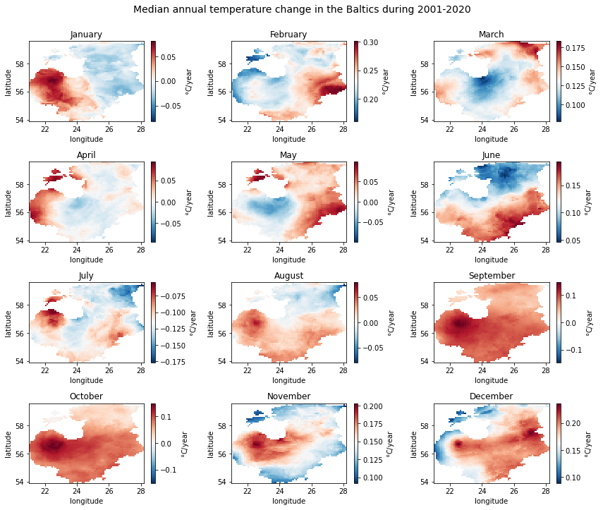
    spatial_ref  int32 0

xarray.DataArray

'month'

• month: 12

• 1 2 3 4 5 6 7 8 9 10 11 12

  array([ 1,  2,  3,  4,  5,  6,  7,  8,  9, 10, 11, 12], dtype=int64)

• Coordinates: (2)
  • month
    (month)
    int64
    1 2 3 4 5 6 7 8 9 10 11 12

    array([ 1,  2,  3,  4,  5,  6,  7,  8,  9, 10, 11, 12], dtype=int64)

  • spatial_ref
    ()
    int32
    0

    crs_wkt :

    GEOGCS["WGS 84",DATUM["WGS_1984",SPHEROID["WGS 84",6378137,298.257223563,AUTHORITY["EPSG","7030"]],AUTHORITY["EPSG","6326"]],PRIMEM["Greenwich",0,AUTHORITY["EPSG","8901"]],UNIT["degree",0.0174532925199433,AUTHORITY["EPSG","9122"]],AXIS["Latitude",NORTH],AXIS["Longitude",EAST],AUTHORITY["EPSG","4326"]]

    semi_major_axis :

    6378137.0

    semi_minor_axis :

    6356752.314245179

    inverse_flattening :

    298.257223563

    reference_ellipsoid_name :

    WGS 84

    longitude_of_prime_meridian :

    0.0

    prime_meridian_name :

    Greenwich

    geographic_crs_name :

    WGS 84

    grid_mapping_name :

    latitude_longitude

    spatial_ref :

    GEOGCS["WGS 84",DATUM["WGS_1984",SPHEROID["WGS 84",6378137,298.257223563,AUTHORITY["EPSG","7030"]],AUTHORITY["EPSG","6326"]],PRIMEM["Greenwich",0,AUTHORITY["EPSG","8901"]],UNIT["degree",0.0174532925199433,AUTHORITY["EPSG","9122"]],AXIS["Latitude",NORTH],AXIS["Longitude",EAST],AUTHORITY["EPSG","4326"]]

    array(0)

• Attributes: (0)

For plotting monthly slope values indicating the intensity of temperature change, we will create a Matplotlib figure object fig consisting of a $4\times 3$ grid of axes.

While iterating over each of the 12 months and their corresponding axes we * will select the corresponding dataset slice from temp_array using the sel command * plot the slope values for that particular month * have a colorbar next to the subplots showing the magnitude of temperature change

# Degree symbol for colorbar
degree_symbol = '$\degree$'

# Create figure and iterate over months to plot slope values in cells
fig, axes = plt.subplots(4, 3, figsize=(12, 10))
for month, ax in zip(months, axes.flatten()):
    ds = temp_array.sel(month=month) # select the month
    ds['slope'].plot(ax=ax, cmap='RdBu_r', cbar_kwargs={'label': '{}C/year'.format(degree_symbol)}) # plot slope values
    month_name = calendar.month_name[int(month)] # get month name
    ax.set_title(month_name)

# Add the title
fig_title = 'Median annual temperature change in the Baltics during 2001-2020'
fig.suptitle(fig_title, y=1, size=14)

# Reduce whitespace around the plot
fig.tight_layout()

For setting the range of the colorbar, we need to know the full range of slope values in the data by checking the minimum and maximum values.

display(temp_array['slope'].min())
display(temp_array['slope'].max())

<xarray.DataArray 'slope' ()>
array(-0.17666797)
Coordinates:
    spatial_ref  int32 0

xarray.DataArray

'slope'

• -0.1767

  array(-0.17666797)

• Coordinates: (1)
  • spatial_ref
    ()
    int32
    0

    crs_wkt :

    GEOGCS["WGS 84",DATUM["WGS_1984",SPHEROID["WGS 84",6378137,298.257223563,AUTHORITY["EPSG","7030"]],AUTHORITY["EPSG","6326"]],PRIMEM["Greenwich",0,AUTHORITY["EPSG","8901"]],UNIT["degree",0.0174532925199433,AUTHORITY["EPSG","9122"]],AXIS["Latitude",NORTH],AXIS["Longitude",EAST],AUTHORITY["EPSG","4326"]]

    semi_major_axis :

    6378137.0

    semi_minor_axis :

    6356752.314245179

    inverse_flattening :

    298.257223563

    reference_ellipsoid_name :

    WGS 84

    longitude_of_prime_meridian :

    0.0

    prime_meridian_name :

    Greenwich

    geographic_crs_name :

    WGS 84

    grid_mapping_name :

    latitude_longitude

    spatial_ref :

    GEOGCS["WGS 84",DATUM["WGS_1984",SPHEROID["WGS 84",6378137,298.257223563,AUTHORITY["EPSG","7030"]],AUTHORITY["EPSG","6326"]],PRIMEM["Greenwich",0,AUTHORITY["EPSG","8901"]],UNIT["degree",0.0174532925199433,AUTHORITY["EPSG","9122"]],AXIS["Latitude",NORTH],AXIS["Longitude",EAST],AUTHORITY["EPSG","4326"]]

    array(0)

• Attributes: (0)

<xarray.DataArray 'slope' ()>
array(0.30160443)
Coordinates:
    spatial_ref  int32 0

xarray.DataArray

'slope'

• 0.3016

  array(0.30160443)

• Coordinates: (1)
  • spatial_ref
    ()
    int32
    0

    crs_wkt :

    GEOGCS["WGS 84",DATUM["WGS_1984",SPHEROID["WGS 84",6378137,298.257223563,AUTHORITY["EPSG","7030"]],AUTHORITY["EPSG","6326"]],PRIMEM["Greenwich",0,AUTHORITY["EPSG","8901"]],UNIT["degree",0.0174532925199433,AUTHORITY["EPSG","9122"]],AXIS["Latitude",NORTH],AXIS["Longitude",EAST],AUTHORITY["EPSG","4326"]]

    semi_major_axis :

    6378137.0

    semi_minor_axis :

    6356752.314245179

    inverse_flattening :

    298.257223563

    reference_ellipsoid_name :

    WGS 84

    longitude_of_prime_meridian :

    0.0

    prime_meridian_name :

    Greenwich

    geographic_crs_name :

    WGS 84

    grid_mapping_name :

    latitude_longitude

    spatial_ref :

    GEOGCS["WGS 84",DATUM["WGS_1984",SPHEROID["WGS 84",6378137,298.257223563,AUTHORITY["EPSG","7030"]],AUTHORITY["EPSG","6326"]],PRIMEM["Greenwich",0,AUTHORITY["EPSG","8901"]],UNIT["degree",0.0174532925199433,AUTHORITY["EPSG","9122"]],AXIS["Latitude",NORTH],AXIS["Longitude",EAST],AUTHORITY["EPSG","4326"]]

    array(0)

• Attributes: (0)

We will create a colorbar normalization object called divnorm to set the range. Using the TwoSlopeNorm command and setting the parameters vmin=-0.2 and vmax=0.4 should cover the range of slope values. As our colorbar is diverging, we also need to set vcenter=0.

divnorm = mcolors.TwoSlopeNorm(vmin=-0.2, vcenter=0, vmax=0.4)

We can now recreate the plot with our custom colorbar range by specifying the norm parameter.

# Degree symbol for colorbar
degree_symbol = '$\degree$'

# Create figure and iterate over months to plot slope values in cells
fig, axes = plt.subplots(4, 3, figsize=(12, 10))
for month, ax in zip(months, axes.flatten()):
    ds = temp_array.sel(month=month) # select the month
    ds['slope'].plot(ax=ax, cmap='RdBu_r', norm=divnorm, cbar_kwargs={'label': '{}C/year'.format(degree_symbol)}) # plot slope values with custom colorbar range
    month_name = calendar.month_name[int(month)] # get month name
    ax.set_title(month_name)

# Add the title
fig_title = 'Median annual temperature change in the Baltics during 2001-2020'
fig.suptitle(fig_title, y=1, size=14)

# Reduce whitespace around the plot
fig.tight_layout()

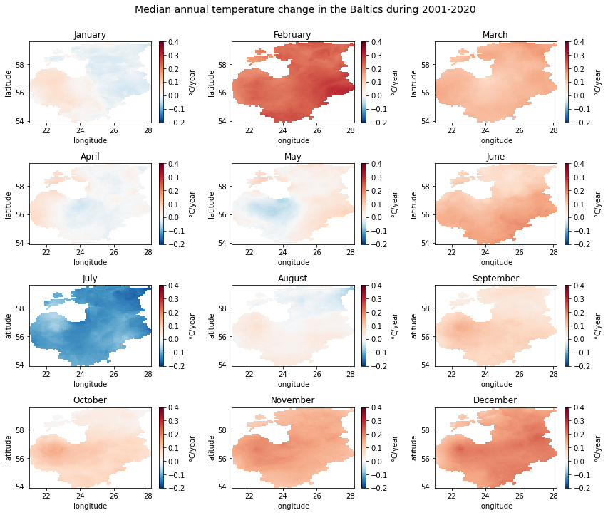
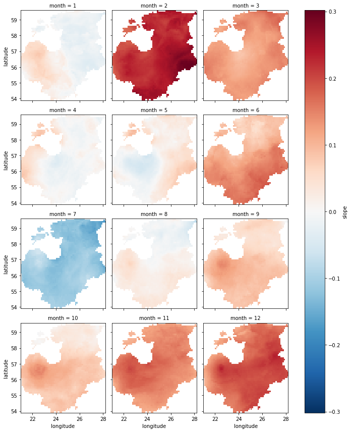
From the plots we can see that majority of the months show an increasing trend, which is the strongest in February and December. Although parts of the Baltics show a slight decreasing trend in other months (e.g. the western part in January), the only month with a clear decreasing trend is July. No clear spatial pattern exists in the detected significant trend locations.

Plotting significant trends

As we examined above when printing out detected significant trend counts per month, only some grid cells indicated significant trends in the study period. We could also see that the three possible trend classes—decreasing, no trend and increasing— are not present in the case of some months.

To see whether the temperature changes seen in the previous plot were also statistically significant, we will now plot the numeric_trend variable. We will use the three numeric trend classes to set the colorbar. To avoid getting unnecessary ticks in the colorbar, we need to specify the corresponding parameter in cbar_kwargs.

# Set colorbar range
divnorm = mcolors.TwoSlopeNorm(vmin=-1, vcenter=0, vmax=1)

# Colormap
colors = ['#A89355', '#C8C9CA', '#65C39E']
cmap = matplotlib.colors.ListedColormap(colors)

# Create figure and iterate over months to plot significance of trends in cells
fig, axes = plt.subplots(4, 3, figsize=(12, 10))
for month, ax in zip(months, axes.flatten()):
    ds = temp_array.sel(month=month) # select month
    ds['numeric_trend'].plot(ax=ax, norm=divnorm, cmap=cmap, cbar_kwargs={'ticks': [-1, 0, 1], 'label': '{}C/year'.format(degree_symbol)}) # plot trends
    month_name = calendar.month_name[int(month)] # get month name
    ax.set_title(month_name)

# Add the title
fig_title = 'Significance of temperature trends in the Baltics during 2001-2020'
fig.suptitle(fig_title, y=1, size=14)

# Reduce whitespace around the plot
fig.tight_layout()

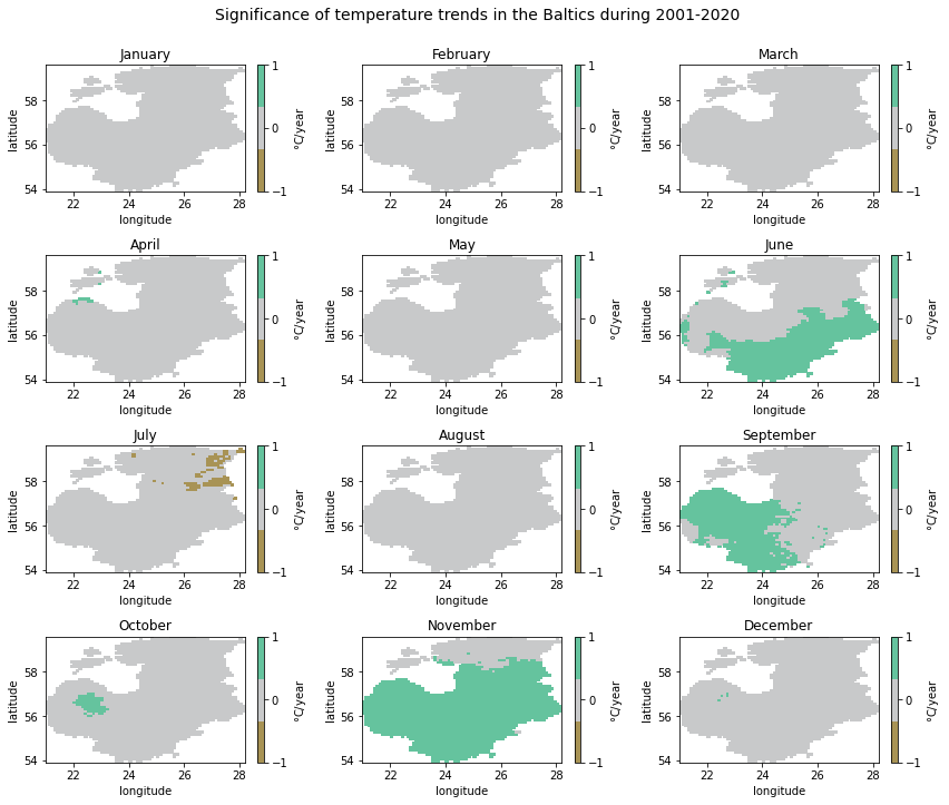
Although there is no clear temporal or spatial pattern in the significant trends detected, we can see that increasing trends were mostly present in the southern half of the study area, i.e. Latvia and Lithuania. In November, significant increasing trends also reached southern Estonia. The only significant decreasing trends were detected in July, particularly in the eastern part of Estonia.

Perhaps somewhat surprisingly, the winter months with the highest slope values—February and December— did not show up as significant trends.

Automatic plotting

We have now learned to plot the hard way by customizing the figures manually. Xarray and Matplotlib can actually do certain things for us when plotting, so that quick plots can be displayed with a single line of code.

For this, we use the imshow command and specify the coordinates with longitude and latitude. The col parameter make sure that we get a plot for each month. Parameter col_wrap tells Matplotlib to plot three months per row.

# Plot monthly slope values automatically
temp_array['slope'].plot.imshow('longitude', 'latitude', col='month', col_wrap=3)

<xarray.plot.facetgrid.FacetGrid at 0x14acb42f448>

References

• Atta-ur-Rahman, and Dawood, M. (2017). Spatio-statistical analysis of temperature fluctuation using Mann–Kendall and Sen’s slope approach. Clim. Dyn. 48, 783–797. doi:10.1007/s00382-016-3110-y.

• Cornes, R. C., van der Schrier, G., van den Besselaar, E. J. M., and Jones, P. D. (2018). An Ensemble Version of the E-OBS Temperature and temperature Data Sets. J. Geophys. Res. Atmos. 123, 9391–9409. doi:10.1029/2017JD028200.

• Jaagus, J., Sepp, M., Tamm, T., Järvet, A., and Mõisja, K. (2017). Trends and regime shifts in climatic conditions and river runoff in Estonia during 1951–2015. Earth Syst. Dyn. 8, 963–976. doi:10.5194/esd-8-963-2017.

• Kendall, M. G. (1957). Rank Correlation Methods. Biometrika 44, 298. doi:10.2307/2333282.

• Mann, H. B. (1945). Non-Parametric Test Against Trend. Econometrica 13, 245–259. Available at: http://www.economist.com/node/18330371?story%7B_%7Did=18330371.

• Sen Pranab Kumar (1968). Estimates of the Regression Coefficient Based on Kendall’s Tau. J. Am. Stat. Assoc. 63, 1379–1389.

• Silva Junior, C. H. L., Almeida, C. T., Santos, J. R. N., Anderson, L. O., Aragão, L. E. O. C., and Silva, F. B. (2018). Spatiotemporal rainfall trends in the Brazilian legal Amazon between the years 1998 and 2015. Water (Switzerland) 10, 1–16. doi:10.3390/w10091220.

previous

Test that everything works

next

FAIR and Reproducible Research